Chapter 12 — Linear Programming | Mathematics Class XII

12.1 Introduction

In earlier classes, we have discussed systems of linear equations and their applications. In Class XI, we studied linear inequalities and systems of linear inequalities in two variables and their solutions by graphical method.

Many applications in mathematics involve systems of inequalities/equations. In this chapter, we shall apply systems of linear inequalities to solve real-life problems of the type below:

Example — Furniture Dealer

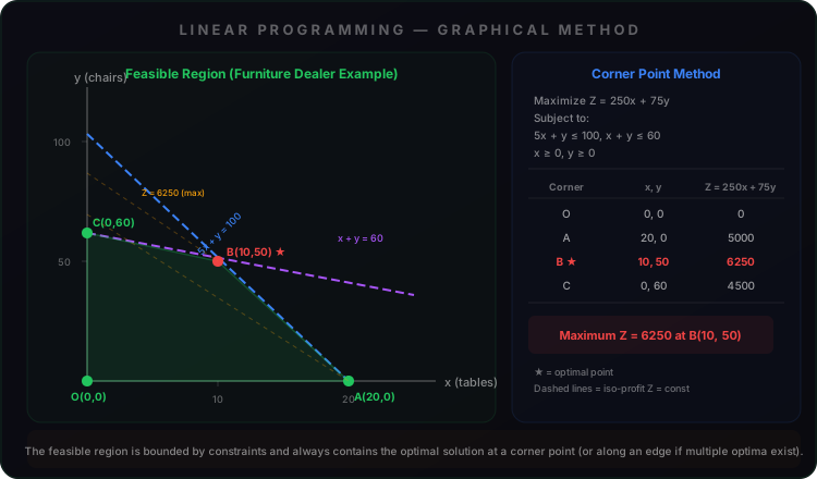
A furniture dealer deals in only two items — tables and chairs. He has ₹50,000 to invest and has storage space of at most 60 pieces. A table costs ₹2,500 and a chair ₹500. He estimates that from the sale of one table he can make a profit of ₹250 and from one chair ₹75. How many tables and chairs should he buy to maximise his total profit?

Such problems which seek to maximise (or minimise) profit (or cost) form a general class of problems called optimisation problems. A special but very important class of optimisation problems is linear programming. Linear programming problems are of much interest because of their wide applicability in industry, commerce, management science, etc.

12.2 Linear Programming Problem and its Mathematical Formulation

We begin with the furniture dealer example, which leads to the mathematical formulation of a problem in two variables.

Mathematical Formulation

Let x be the number of tables and y be the number of chairs. Then:

Decision variables & constraints x \geq 0, y \geq 0 (non-negative constraints) 2500x + 500y \leq 50000 \to 5x + y \leq 100 (investment constraint) x + y \leq 60 (storage constraint) Objective function (maximise) Z = 250x + 75y

The dealer wants to find the values of x and y that maximise Z = 250x + 75y subject to the above constraints. This is a linear programming problem (LPP).

Figure 12.1 — Feasible region with corner points (left) and evaluation table (right). Optimal solution at B(10, 50) with Z = 6250.

Corner Point Method

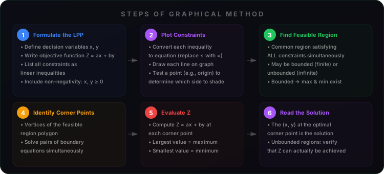
Six steps of the graphical method for solving LPP

Figure 12.2 — Six steps of the graphical method for solving a linear programming problem

The method of solving a linear programming problem by graphing the constraints and testing the corner points of the feasible region is called the corner point method. The fundamental theorem states:

Fundamental Theorem of Linear Programming

If the feasible region is bounded, then the objective function Z has both a maximum and a minimum value, and these occur at the corner points of the feasible region. If the feasible region is unbounded, the objective function may or may not have a maximum or minimum value — further analysis is needed.

Types of LPP

bounded

Bounded Feasible Region

The feasible region is a closed polygon. Both maximum and minimum of Z exist and occur at corner points.

∞

Unbounded Feasible Region

The feasible region extends infinitely in some direction. Z may not have a maximum or minimum — must verify by checking whether Z can exceed a given value.

Multiple Optima

If the objective function Z has the same maximum (or minimum) value at two corner points, then every point on the line segment joining these two points gives the same maximum (or minimum) value. In this case, the LPP has infinitely many optimal solutions.

Diet Problem Example

A dietician wishes to combine two foods, F₁ and F₂, such that the mixture contains at least 80 units of vitamin A and 100 units of vitamin B. Food F₁ costs ₹4/unit and F₂ costs ₹6/unit. F₁ contains 3 units of vitamin A and 5 units of vitamin B per unit; F₂ contains 5 units of vitamin A and 4 units of vitamin B per unit.

Diet Problem Formulation Minimise Z = 4x₁ + 6x₂ Subject to: 3x₁ + 5x₂ \geq 80 (vitamin A) 5x₁ + 4x₂ \geq 100 (vitamin B) x₁, x₂ \geq 0 Optimal: x₁ = 200/7, x₂ = 200/7, Z \approx ₹108.57 (minimum)

Important note

In this chapter, we study linear programming problems and their solutions by graphical method only, though there are many other methods (such as the simplex method) to solve more complex LPPs.

∑ Summary

A linear programming problem is one that is concerned with finding the optimal value (maximum or minimum) of a linear function of several variables (called the objective function) subject to the conditions that the variables are non-negative and satisfy a set of linear inequalities (called linear constraints).
Variables are sometimes called decision variables and are non-negative.
The corner point method involves finding the feasible region, identifying its corner points, and evaluating the objective function at each corner point to find the optimal value.
If the feasible region is bounded, the objective function attains both maximum and minimum at corner points.
If the feasible region is unbounded, the objective function may or may not have a maximum or minimum — further verification is required.
If Z has the same optimal value at two corner points, then every point on the line segment joining them is also optimal (infinitely many solutions).

📜 Historical Note

George B. Dantzig

1914 – 2005

In World War II, when war operations had to be planned to economise expenditure and maximise damage to the enemy, linear programming problems came to the forefront.

The first problem in linear programming was formulated in 1941 by the Russian mathematician L. Kantorovich and the American economist F. L. Hitchcock, both of whom worked at it independently of each other. This was the well-known transportation problem.

In 1945, the English economist G. Stigler described yet another linear programming problem — that of determining an optimal diet.

In 1947, the American economist G. B. Dantzig suggested an efficient method known as the simplex method — an iterative procedure to solve any linear programming problem in a finite number of steps.

L. Kantorovich and the American mathematical economist T. C. Koopmans were awarded the Nobel Prize in 1975 in Economics for their pioneering work in linear programming. With the advent of computers and necessary software, it has become possible to apply linear programming models to increasingly complex problems in many areas.