Probability
The mathematics of uncertainty — from conditional chance to Bayes' reasoning
In this chapter
13.1 Introduction
The theory of probability was developed to analyse situations where the outcome of an experiment is uncertain. In Class XI, we studied the axiomatic approach to probability and concepts like sample space, events, and probability of events.
In this chapter, we take this forward and study conditional probability, which asks: what is the probability of an event given that another event has already occurred? This leads to important results like the multiplication theorem, the theorem of total probability, and the celebrated Bayes' theorem.
13.2 Conditional Probability
The conditional probability of an event E, given the occurrence of the event F, is defined as:
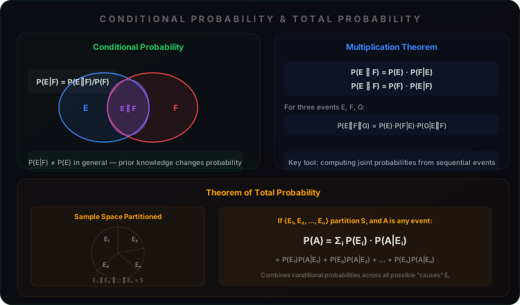
0 ≤ P(E|F) ≤ 1 | P(E'|F) = 1 − P(E|F)
P((E ∪ F)|G) = P(E|G) + P(F|G) − P((E ∩ F)|G)
Theorem of Total Probability
If {E₁, E₂, ..., Eₙ} is a partition of the sample space S (meaning the Eᵢ are pairwise disjoint and their union is S), and each Eᵢ has nonzero probability, then for any event A associated with S:
P(A) = Σᵢ P(Eᵢ) · P(A|Eᵢ)
This theorem allows us to compute P(A) by considering all possible "causes" Eᵢ that could lead to event A, weighting each conditional probability P(A|Eᵢ) by the probability P(Eᵢ) of that cause.
13.3 Multiplication Theorem on Probability
The multiplication theorem provides a way to compute the probability of the intersection of events:
For three events E, F, G:
To find the probability that both E and F occur, we can first find the probability that E occurs, and then multiply by the probability that F occurs given that E has already occurred. This is particularly useful for sequential experiments.
13.4 Independent Events
Two events E and F are said to be independent if the occurrence of one does not affect the probability of occurrence of the other. Mathematically:
Equivalent conditions (when P(E) ≠ 0, P(F) ≠ 0):
P(E|F) = P(E) and P(F|E) = P(F)
Mutually Exclusive vs Independent
Mutually exclusive: E ∩ F = ∅ (cannot both occur).
Independent: P(E ∩ F) = P(E)·P(F) (occurrence of one doesn't affect the other).
These are very different concepts!
Independent vs Pairwise Independent
Events E₁, E₂, ..., Eₙ are independent if P(Eᵢ₁ ∩ ... ∩ Eᵢₖ) = P(Eᵢ₁)·...·P(Eᵢₖ) for every subset. Pairwise independence is weaker than full independence.
13.5 Bayes' Theorem
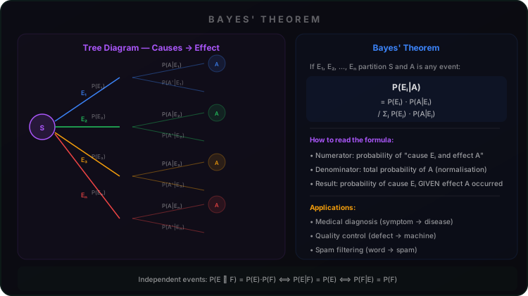
If E₁, E₂, ..., Eₙ are events which constitute a partition of sample space S (i.e., they are pairwise disjoint and E₁ ∪ E₂ ∪ ... ∪ Eₙ = S), and A is any event with nonzero probability, then:
= P(Eᵢ) · P(A|Eᵢ) / P(A)
Numerator: probability of "cause Eᵢ AND effect A" — the joint probability that Eᵢ is the cause and A is the observed effect.
Denominator: the total probability of A — obtained from the theorem of total probability, serving as a normalising constant.
Result: the posterior probability P(Eᵢ|A) — the probability that Eᵢ is the cause, given that we have observed effect A.
Applications of Bayes' Theorem
- Medical diagnosis: Given a positive test result, what is the probability the patient has the disease?
- Quality control: A defective item is found — which machine produced it?
- Spam filtering: Given certain words in an email, what is the probability it is spam?
- Bayesian inference: Updating prior beliefs with new evidence — the foundation of modern statistical reasoning.
∑ Summary
- The conditional probability of an event E, given the occurrence of event F, is P(E|F) = P(E ∩ F)/P(F), P(F) ≠ 0.
- 0 ≤ P(E|F) ≤ 1, and P(E'|F) = 1 − P(E|F).
- P((E ∪ F)|G) = P(E|G) + P(F|G) − P((E ∩ F)|G).
- Multiplication theorem: P(E ∩ F) = P(E) · P(F|E) = P(F) · P(E|F).
- For independent events E and F: P(E ∩ F) = P(E) · P(F), P(E|F) = P(E), P(F|E) = P(F).
- Theorem of total probability: If {E₁, E₂, ..., Eₙ} partition S, then P(A) = Σᵢ P(Eᵢ) · P(A|Eᵢ).
- Bayes' theorem: P(Eᵢ|A) = P(Eᵢ) · P(A|Eᵢ) / Σⱼ P(Eⱼ) · P(A|Eⱼ).
- Bayes' theorem converts "probability of cause given effect" into "probability of effect given cause" — enabling posterior inference from observed evidence.
📜 Historical Note
The great Dutch scientist Christiaan Huygens (1629–1695), became acquainted with the correspondence between Pascal and Fermat and published the first book on probability, De Ratiociniis in Ludo Aleae, containing solutions of many interesting problems on probability in games of chance.
The next great work on probability theory is by Jacob Bernoulli (1654–1705), in the form of a great book, Ars Conjectandi, published posthumously in 1713. To him is due the discovery of one of the most important probability distributions — the Binomial distribution.
The next remarkable work on probability lies in 1933. A. N. Kolmogorov (1903–1987) is credited with the axiomatic theory of probability. His book, Foundations of Probability, published in 1933, introduces probability as a set function and is considered a classic.