Continuity and Differentiability
The twin pillars of calculus — when functions flow smoothly and when they don't
In this chapter
5.1 Introduction
"The whole of science is nothing more than a refinement of everyday thinking." — Albert Einstein
This chapter extends our study of differentiation from Class XI. We introduce the fundamental concepts of continuity and differentiability, learn to differentiate inverse trigonometric functions, and explore exponential and logarithmic functions. These concepts lead to powerful techniques of differentiation and reveal deep connections between smoothness of a function and its rate of change.
5.2 Continuity
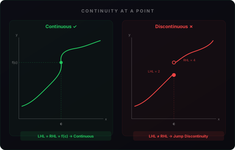
A function is continuous at a point if its graph can be drawn through that point without lifting the pen. More precisely:
A function f is continuous at x = c if:
1. f(c) is defined
2. lim[x→c] f(x) exists
3. lim[x→c] f(x) = f(c)
This means: LHL = RHL = f(c)
Types of Discontinuity
Removable
LHL = RHL but ≠ f(c) or f(c) undefined. A single "hole" in the graph that can be patched.
Jump
LHL ≠ RHL. The function "jumps" to a different value. The gap cannot be bridged.
Infinite
LHL or RHL → ±∞. A vertical asymptote. The function grows without bound.
Continuous
LHL = RHL = f(c). The graph flows smoothly through the point. No lifting required.
Algebra of Continuous Functions
If f and g are continuous at x = c, then:
(i) f ± g is continuous at x = c
(ii) f · g is continuous at x = c
(iii) λf is continuous (for constant λ)
(iv) f/g is continuous at x = c (provided g(c) ≠ 0)
Continuity of Standard Functions
- Polynomial functions are continuous everywhere
- Rational functions are continuous in their domain
- Trigonometric functions (sin, cos, tan) are continuous in their domain
- Exponential functions (eˣ, aˣ) are continuous everywhere
- Logarithmic functions are continuous in their domain
If g is continuous at c and f is continuous at g(c), then f ∘ g is continuous at c.
Example: sin(x²) is continuous because sin and x² are both continuous everywhere.
5.3 Differentiability
A function is differentiable at a point if its derivative exists there — geometrically, if a unique tangent can be drawn at that point.
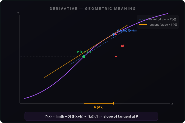
f'(x) = lim[h→0] [f(x+h) − f(x)] / h
If this limit exists, f is differentiable at x. Geometrically, f'(x) = slope of the tangent line at x.
Theorem: Differentiability implies Continuity
If f is differentiable at x = c, then f is continuous at x = c.
The converse is NOT true! The function f(x) = |x| is continuous at x = 0 but NOT differentiable there (sharp corner).
Chain Rule
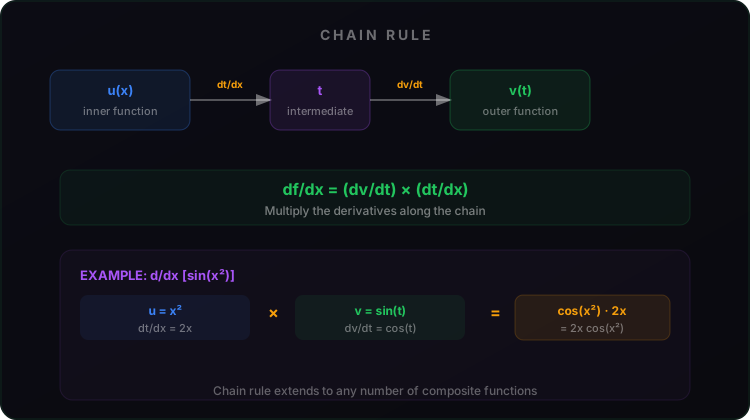
The chain rule is the workhorse of differentiation — it lets us differentiate composite functions.
Implicit Differentiation
When y is defined implicitly by an equation (not as y = f(x)), differentiate both sides w.r.t. x using chain rule whenever y appears:
Standard Derivatives
| Function | Derivative |
|---|---|
| sin⁻¹ x | 1 / √(1 − x²) |
| cos⁻¹ x | −1 / √(1 − x²) |
| tan⁻¹ x | 1 / (1 + x²) |
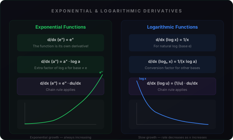
| eˣ | eˣ |
| aˣ | aˣ log a |
| log x | 1/x |
Second Order Derivatives
The second derivative f''(x) = d/dx[f'(x)] measures the rate of change of the rate of change — concavity of the curve.
5.4 Exponential and Logarithmic Functions
Exponential and logarithmic functions are inverses of each other and have beautifully simple derivatives.
Logarithmic Differentiation
For functions of the form f(x) = [u(x)]ᵛ⁽ˣ⁾, take logarithm on both sides first, then differentiate implicitly:
log y = v(x) · log u(x)
(1/y)(dy/dx) = v'(x) log u(x) + v(x) · u'(x)/u(x)
dy/dx = y × [v' log u + v · u'/u]
(i) Functions of the form [f(x)]ᵍ⁽ˣ⁾ (variable raised to variable)
(ii) Products of many factors: y = f₁ · f₂ · ... · fₙ
(iii) Quotients of many factors
Note: Both f(x) and u(x) must be positive for this technique.
5.5 Mean Value Theorem
The Mean Value Theorem (MVT) connects the average rate of change over an interval to the instantaneous rate of change at some point within that interval.
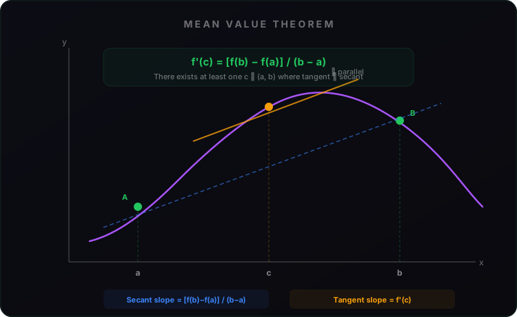
If f is continuous on [a, b] and differentiable on (a, b), then there exists at least one c ∈ (a, b) such that:
f'(c) = [f(b) − f(a)] / (b − a)
Geometrically: the tangent at some point is parallel to the chord joining (a, f(a)) and (b, f(b)).
If f is continuous on [a, b], differentiable on (a, b), and f(a) = f(b), then there exists c ∈ (a, b) where f'(c) = 0.
Rolle's Theorem is MVT with equal endpoint values — the tangent is horizontal.
5.6 Summary
• Continuity: lim[x→c] f(x) = f(c) — no jumps, holes, or breaks
• Discontinuity types: removable, jump, infinite
• Sum, difference, product, quotient of continuous functions are continuous
• Differentiability: f'(x) exists — unique tangent at every point
• Differentiable ⟹ Continuous, but NOT the reverse
• Chain rule: d/dx [f(g(x))] = f'(g(x)) · g'(x)
• Standard derivatives: sin⁻¹x → 1/√(1−x²), eˣ → eˣ, log x → 1/x, etc.
• Logarithmic differentiation: for [u(x)]ᵛ⁽ˣ⁾, take log first, then differentiate
• MVT: f'(c) = [f(b)−f(a)]/(b−a) — tangent ∥ secant at some c
• Rolle's: special case of MVT when f(a) = f(b) → f'(c) = 0