Statistics
Measuring how data spreads — from simple range to powerful standard deviation
In this chapter
13.1 Measures of Dispersion
"Statistics may be rightly called the science of averages and their estimates." — A.L. Bowley & A.L. Boddington
Measures of central tendency (mean, median, mode) tell us where data clusters, but they don't tell us how spread out the data is. Two datasets can have the same mean but very different spreads!
Batsman A: 30, 91, 0, 64, 42, 80, 30, 5, 117, 71 → Mean = 53
Batsman B: 53, 46, 48, 50, 53, 53, 58, 60, 57, 52 → Mean = 53
Same mean! But Batsman A is wildly inconsistent (0 to 117), while Batsman B is steady (46 to 60). We need measures of dispersion to capture this difference.
Types of Dispersion Measures
Range
Maximum - Minimum. Simple but only uses two values.
Mean Deviation
Average of absolute deviations from mean or median.
Variance
Average of squared deviations from mean. Uses all data points.
Standard Deviation
Square root of variance. Most widely used measure.
13.2 Range
The range is the simplest measure of dispersion — just the difference between the maximum and minimum values.
Range = Maximum value - Minimum value
Example: For Batsman A (0, 5, 30, 30, 42, 64, 71, 80, 91, 117)
Range = 117 - 0 = 117
For Batsman B (46, 48, 50, 52, 53, 53, 53, 57, 58, 60)
Range = 60 - 46 = 14
• Only uses 2 values (max and min), ignores all others
• Very sensitive to outliers
• Doesn't tell us how data is distributed between extremes
• Same range can mean very different distributions
13.3 Mean Deviation
The mean deviation measures the average distance of data points from a central value (mean or median). We use absolute values to avoid negative deviations canceling positive ones.
Steps to Calculate Mean Deviation
Step 1: Calculate the mean (x̄) or median (M)
Step 2: Find deviations: xᵢ - x̄ or xᵢ - M
Step 3: Take absolute values: |xᵢ - x̄|
Step 4: Find the mean of absolute deviations
M.D.(x̄) = Σ|xᵢ - x̄| / n
M.D.(M) = Σ|xᵢ - M| / n
For Ungrouped Data
Data: 6, 7, 10, 12, 13, 4, 8, 12
Mean = 72/8 = 9
|6-9|=3, |7-9|=2, |10-9|=1, |12-9|=3, |13-9|=4, |4-9|=5, |8-9|=1, |12-9|=3
M.D.(x̄) = (3+2+1+3+4+5+1+3)/8 = 22/8 = 2.75
For Grouped Data (Discrete)
M.D.(x̄) = Σfᵢ|xᵢ - x̄| / N, where N = Σfᵢ
Multiply each absolute deviation by its frequency, sum them all, divide by total frequency.
For Grouped Data (Continuous)
Use the mid-point of each class interval as xᵢ, then apply the same formula as discrete data.
Class 10-20 → mid-point = 15
Class 20-30 → mid-point = 25
• Uses absolute values, which breaks algebraic properties
• Cannot be used for further mathematical analysis
• Not as statistically powerful as variance/standard deviation
13.4 Variance and Standard Deviation
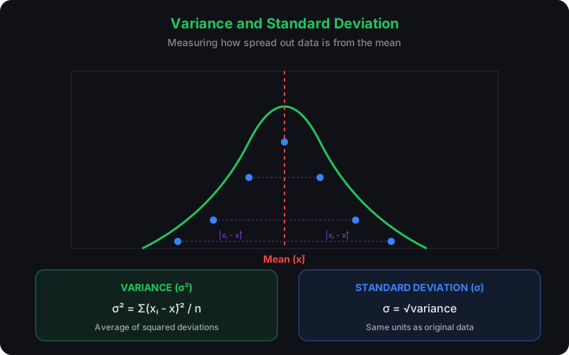
Instead of absolute values, we can square the deviations to eliminate negatives. The average of squared deviations is called variance.
Variance
σ² = Σ(xᵢ - x̄)² / n
Variance is always ≥ 0. If variance = 0, all values are identical.
Units: squared units of original data (e.g., if data in meters, variance in m²)
Standard Deviation
σ = √(variance) = √[Σ(xᵢ - x̄)² / n]
Standard deviation has the same units as the original data.
It's the most widely used measure of dispersion!
Why Standard Deviation?
Uses All Data
Every data point contributes to the calculation.
Algebraic Properties
Can be used in further mathematical analysis and statistical tests.
Same Units
Same units as original data, making it interpretable.
Foundation for Statistics
Basis for confidence intervals, hypothesis testing, and more.
For Frequency Distributions
σ² = Σfᵢ(xᵢ - x̄)² / N, where N = Σfᵢ
σ = √[Σfᵢ(xᵢ - x̄)² / N]
Use mid-points of class intervals as xᵢ, then apply the discrete formula.
Alternative formula:
σ² = [Σfᵢxᵢ² / N] - (x̄)²
This avoids calculating deviations directly!
13.5 Shortcut Method
When data values are large, calculating mean and variance directly is tedious. The step-deviation method simplifies calculations.
Step-Deviation Method
Let A = assumed mean, h = class width
yᵢ = (xᵢ - A) / h (step deviations)
Then:
x̄ = A + h × (Σfᵢyᵢ / N)
σ² = h² × [Σfᵢyᵢ² / N - (Σfᵢyᵢ / N)²]
• Reduces large numbers to small integers
• Makes multiplication and addition easier
• Choose A near the middle of data for best results
• Same formula works for both discrete and continuous data
Properties of Variance and SD
1. Adding a constant to all values: variance unchanged
2. Multiplying all values by k: variance becomes k²σ², SD becomes kσ
3. Variance ≥ 0 always
4. Variance = 0 iff all values are equal
13.6 Summary
• Range: Max - Min. Simple but limited.
• Mean Deviation: M.D. = Σ|xᵢ - x̄| / n. Uses absolute values.
• Variance: σ² = Σ(xᵢ - x̄)² / n. Average squared deviation.
• Standard Deviation: σ = √variance. Most important measure.
• For frequency data: Replace n with N = Σfᵢ, use fᵢ weighting.
• Shortcut method: Use step-deviations yᵢ = (xᵢ - A)/h to simplify calculations.
• Adding constant: Doesn't affect variance/SD.
• Multiplying by k: Variance × k², SD × k.