Structure of Atom
From subatomic particles to quantum mechanics — understanding the building blocks of matter
In this chapter
- Discovery of Subatomic Particles
- Thomson's Model of the Atom
- Rutherford's Nuclear Model
- Bohr's Model of the Atom
- Dual Behaviour of Matter
- Heisenberg Uncertainty Principle
- Quantum Mechanical Model
- Orbitals & Quantum Numbers
- Shapes of Orbitals
- Energies of Orbitals
- Filling of Orbitals — Rules
- Electronic Configuration
- Stability of Half-filled & Fully-filled Subshells
- Summary
2.1 Discovery of Subatomic Particles
By the end of the 19th century, atoms were considered indivisible particles. However, the discovery of subatomic particles changed this view entirely.
Electron — J.J. Thomson (1897)
Thomson passed electric current through cathode ray tubes at low pressure and observed the properties of cathode rays. He concluded that cathode rays are streams of negatively charged particles (electrons) that are emitted from the cathode and travel towards the anode.
Properties of Cathode Rays:
- They travel in straight lines and cast shadows of objects placed in their path.
- They are deflected by electric and magnetic fields, proving they carry negative charge.
- They produce fluorescence on zinc sulphide screens.
- Their charge-to-mass ratio (e/m) is independent of the gas in the tube and the material of the electrode.
For cathode ray particles: e/m = 1.7588 × 10¹¹ C/kg
This value is constant regardless of the gas used or the electrode material, proving that electrons are fundamental particles present in all atoms.
Proton — Goldstein (1886)
In the discharge tube experiment, Goldstein observed canal rays — positively charged rays traveling in the opposite direction to cathode rays. These were found to consist of positively charged particles called protons. The charge-to-mass ratio of canal rays depends on the gas used.
Neutron — James Chadwick (1932)
Chadwick bombarded beryllium with alpha particles and observed an uncharged radiation. This radiation was made up of neutral particles called neutrons, each with a mass approximately equal to that of a proton.
2.2 Thomson's Model of the Atom
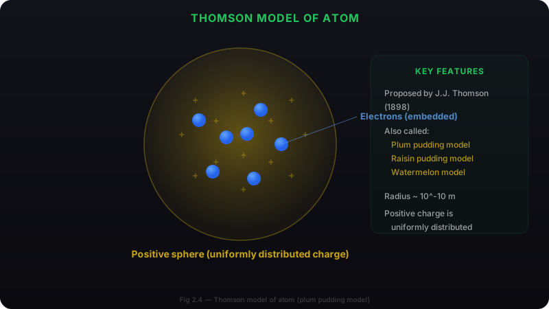
Thomson proposed a model of the atom (1904) that is compared to a plum pudding (or watermelon). In this model:
- The atom is a positively charged sphere of radius ~10⁻¹⁰ m.
- Electrons are uniformly embedded throughout the positive sphere, like seeds in a watermelon.
- The total positive charge equals the total negative charge, making the atom electrically neutral.
Thomson's model could not explain the results of the Rutherford alpha-particle scattering experiment. It also could not explain the atomic spectra observed in emission and absorption studies.
2.3 Rutherford's Nuclear Model of the Atom
Rutherford, along with his students Geiger and Marsden, conducted the famous alpha-particle scattering experiment (1911). They bombarded a thin gold foil (~0.0004 cm thick) with fast-moving alpha particles (He²⁺) and observed the scattering pattern.
Observations
- Most alpha particles passed straight through the gold foil without deflection.
- A small fraction of alpha particles were deflected by small angles.
- A very small number (~1 in 20,000) were deflected by angles greater than 90°, and some were even bounced back (180° deflection).
Conclusions
- Most of the atom is empty space — allowing alpha particles to pass through.
- The positive charge and most of the mass of the atom is concentrated in a very small region called the nucleus.
- The size of the nucleus is ~10⁻¹⁵ m, while the atom is ~10⁻¹⁰ m — the nucleus is about 10,000 times smaller than the atom.
1. According to Maxwell's electromagnetic theory, an accelerated charged particle should continuously lose energy by emitting electromagnetic radiation. The electron would spiral inward and eventually fall into the nucleus — making atoms unstable. But atoms are stable!
2. Rutherford's model could not explain the line spectra of atoms — the characteristic wavelengths emitted by different elements.
2.4 Bohr's Model of the Atom
Neil Bohr (1913) modified Rutherford's model by incorporating early quantum theory. He proposed that electrons revolve around the nucleus in fixed circular paths called orbits or stationary states.
Fixed Orbits
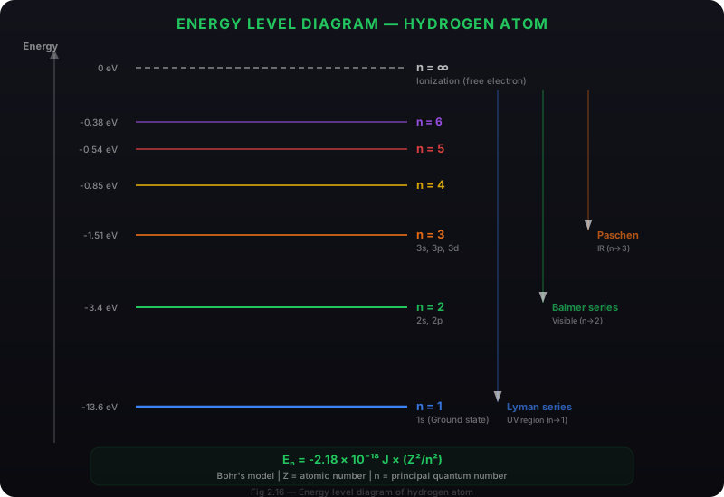
Electrons revolve in specific orbits without radiating energy. Each orbit has a fixed energy and is designated by the quantum number n = 1, 2, 3, ...
Energy Absorption/Emission
Energy is absorbed or emitted only when an electron jumps from one orbit to another — not while revolving in the same orbit.
Key Results of Bohr's Model
- The radius of the nth orbit: rₙ = 0.529 × n²/Z Å (for hydrogen, Z = 1)
- The energy of the electron in the nth orbit: Eₙ = -13.6 × Z²/n² eV (for hydrogen)
- The velocity of the electron in the nth orbit: vₙ = 2.18 × 10⁶ × Z/n m/s
When an electron jumps from a higher orbit (n₂) to a lower orbit (n₁), it emits radiation of a specific frequency:
ν = (E₂ - E₁)/h
This explains the discrete lines in the hydrogen spectrum — the Balmer series (visible region, n→2), Lyman series (UV, n→1), Paschen series (IR, n→3), Brackett (n→4), and Pfund (n→5).
1. It could not explain the spectra of atoms with more than one electron (multi-electron atoms).
2. It could not explain the fine line spectrum of hydrogen (dual lines in Balmer series).
3. It violates the Heisenberg Uncertainty Principle by assuming precise paths for electrons.
4. It could not explain the bonding in molecules or the splitting of spectral lines in a magnetic field (Zeeman effect).
2.5 Dual Behaviour of Matter
Louis de Broglie (1924) proposed that just as light has both wave-like and particle-like properties, matter also exhibits dual behaviour. Moving particles like electrons should have wave-like properties associated with them.
This was experimentally confirmed by Davisson and Germer (1927) through electron diffraction experiments, and independently by G.P. Thomson.
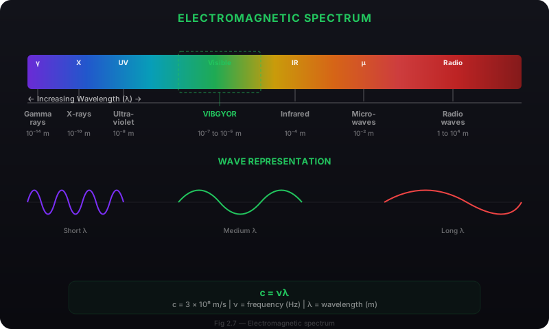
The wave-like behaviour of electrons is significant only at the subatomic level (very small mass). For macroscopic objects, the wavelength is so small that wave behaviour is negligible.
2.6 Heisenberg Uncertainty Principle
Werner Heisenberg (1927) proposed that it is impossible to simultaneously determine both the position and momentum (velocity) of a subatomic particle with absolute accuracy.
This is not a limitation of experimental technique — it is a fundamental property of nature. The more precisely we know the position of a particle, the less precisely we know its momentum, and vice versa.
The Heisenberg Uncertainty Principle directly contradicts Bohr's model, which assumes electrons travel in well-defined circular paths. Since we cannot know both the exact position and velocity of an electron, the concept of a precise orbit is meaningless. This led to the development of the quantum mechanical model.
2.7 Quantum Mechanical Model of the Atom
The quantum mechanical model (also called the wave mechanical model) was developed by Erwin Schrödinger (1926). Instead of precise orbits, it describes electrons as wave functions (ψ) that give the probability of finding an electron in a particular region.
Schrödinger's wave equation for the hydrogen atom is:
The solution of Schrödinger's equation gives a set of wave functions (ψ) called atomic orbitals. Each orbital has a definite energy, shape, and size.
Wave Function (ψ)
ψ has no physical meaning by itself. However, ψ² (the square of the wave function) gives the probability density — the probability of finding an electron per unit volume.
Electron Cloud
The region where the probability of finding the electron is high (>90%) is called the orbital. Electrons are not at fixed positions — they exist as probability clouds.
2.8 Orbitals & Quantum Numbers
An orbital is defined as the region of space around the nucleus where the probability of finding an electron is maximum. Each orbital is described by a set of three quantum numbers. A fourth quantum number (spin) describes the electron itself.
The Four Quantum Numbers
Principal (n)
Determines the size and energy of the orbital. n = 1, 2, 3, ... (positive integers). Higher n → larger orbital, higher energy.
Angular Momentum (l)
Determines the shape of the orbital. l = 0 to (n-1). Values: s (l=0), p (l=1), d (l=2), f (l=3).
Magnetic (mₗ)
Determines the orientation of the orbital in space. mₗ = -l to +l. For p orbital: mₗ = -1, 0, +1 → three orientations (pₓ, pᵧ, pᵤ).
Spin (mₛ)
Describes the spin direction of the electron. mₛ = +½ (spin up) or -½ (spin down). Maximum 2 electrons per orbital.
Table 2.1 — Quantum Numbers and Allowed Values
| Quantum Number | Symbol | Values | What it determines |
|---|---|---|---|
| Principal | n | 1, 2, 3, 4, ... | Size, energy of orbital |
| Angular Momentum | l | 0, 1, 2, ... (n-1) | Shape of orbital |
| Magnetic | mₗ | -l, ..., 0, ..., +l | Orientation in space |
| Spin | mₛ | +½, -½ | Spin direction of electron |
s subshell (l = 0): 1 orbital
p subshell (l = 1): 3 orbitals (pₓ, pᵧ, pᵤ)
d subshell (l = 2): 5 orbitals
f subshell (l = 3): 7 orbitals
2.9 Shapes of Orbitals
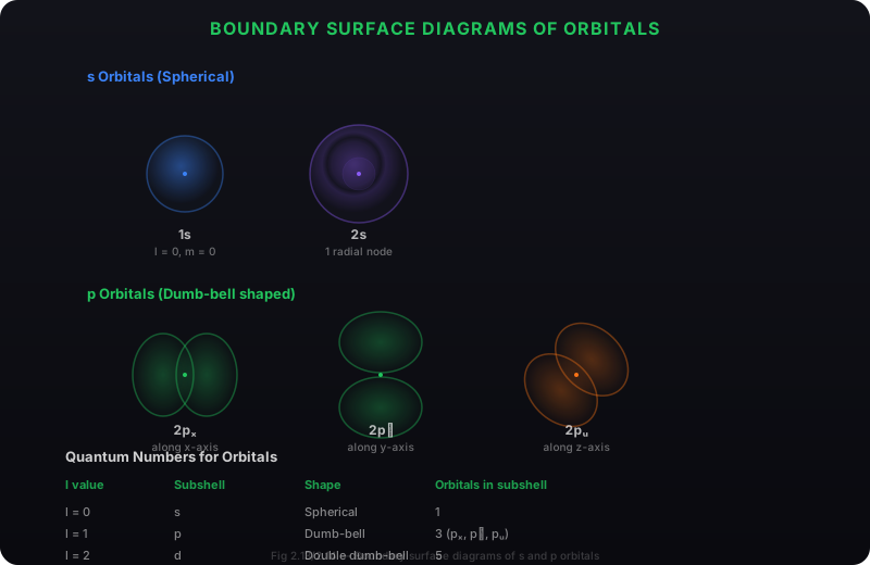
The shapes of orbitals are described by boundary surface diagrams — surfaces within which there is a high probability (~90%) of finding the electron.
s Orbital — Spherical
The s orbital is spherically symmetrical. Its size increases with increasing n (1s < 2s < 3s ...). The 2s orbital has one radial node (a region where probability of finding electron is zero).
p Orbital — Dumb-bell Shaped
The p orbital is dumb-bell shaped with two lobes separated by a nodal plane. There are three p orbitals (2pₓ, 2pᵧ, 2pᵤ) oriented along the x, y, and z axes respectively.
d Orbital — Double Dumb-bell
Five d orbitals exist for each principal energy level (n ≥ 3). Four have a clover-leaf shape and one (dᵤ²) is dumb-bell shaped with a doughnut.
A node is a region where the probability of finding an electron is zero.
Angular node = l (related to shape)
Radial node = n - l - 1 (related to size)
Total nodes = n - 1
2.10 Energies of Orbitals
The energy of an orbital depends on both the principal quantum number (n) and the azimuthal quantum number (l).
In Hydrogen-like Atoms (One-electron species)
For hydrogen and hydrogen-like species (He⁺, Li²⁺, etc.), the energy depends only on n:
In Multi-electron Atoms
Due to shielding and penetration effects, orbitals with the same n but different l have different energies. The order of orbital energies is:
1s < 2s < 2p < 3s < 3p < 4s < 3d < 4p < 5s < 4d < 5p < 6s < 4f < 5d < 6p < 7s < 5f < 6d < 7p
Remember the (n+l) rule: lower (n+l) → lower energy. If (n+l) is same, lower n → lower energy.
2.11 Filling of Orbitals — Rules
Electrons fill orbitals according to three fundamental rules:
Aufbau Principle
Electrons fill orbitals starting from the lowest energy level and progressively moving to higher energy levels. The order follows the (n+l) rule.
Pauli Exclusion Principle
No two electrons in the same atom can have the same set of all four quantum numbers. Each orbital can hold a maximum of 2 electrons with opposite spins.
Hund's Rule
Electrons fill degenerate orbitals singly first (with parallel spins) before pairing. This minimizes electron-electron repulsion and lowers energy.
(n + l) Rule
Lower (n+l) → lower energy. If (n+l) is equal, lower n → lower energy. Example: 4s (n+l=4) fills before 3d (n+l=5).
2.12 Electronic Configuration
The distribution of electrons in various orbitals of an atom is called its electronic configuration. It is written using the orbital notation (e.g., 1s², 2s², 2p⁶, ...).
Electronic Configurations of First 18 Elements
| Z | Element | Configuration | Subshell notation |
|---|---|---|---|
| 1 | H | 1s¹ | — |
| 2 | He | 1s² | — |
| 3 | Li | 1s² 2s¹ | [He] 2s¹ |
| 4 | Be | 1s² 2s² | [He] 2s² |
| 5 | B | 1s² 2s² 2p¹ | [He] 2s² 2p¹ |
| 6 | C | 1s² 2s² 2p² | [He] 2s² 2p² |
| 7 | N | 1s² 2s² 2p³ | [He] 2s² 2p³ |
| 8 | O | 1s² 2s² 2p⁴ | [He] 2s² 2p⁴ |
| 9 | F | 1s² 2s² 2p⁵ | [He] 2s² 2p⁵ |
| 10 | Ne | 1s² 2s² 2p⁶ | [He] 2s² 2p⁶ |
| 11 | Na | 1s² 2s² 2p⁶ 3s¹ | [Ne] 3s¹ |
| 12 | Mg | 1s² 2s² 2p⁶ 3s² | [Ne] 3s² |
| 13 | Al | 1s² 2s² 2p⁶ 3s² 3p¹ | [Ne] 3s² 3p¹ |
| 14 | Si | 1s² 2s² 2p⁶ 3s² 3p² | [Ne] 3s² 3p² |
| 15 | P | 1s² 2s² 2p⁶ 3s² 3p³ | [Ne] 3s² 3p³ |
| 16 | S | 1s² 2s² 2p⁶ 3s² 3p⁴ | [Ne] 3s² 3p⁴ |
| 17 | Cl | 1s² 2s² 2p⁶ 3s² 3p⁵ | [Ne] 3s² 3p⁵ |
| 18 | Ar | 1s² 2s² 2p⁶ 3s² 3p⁶ | [Ne] 3s² 3p⁶ |
• Noble gas shorthand: Use the preceding noble gas in brackets. E.g., Na = [Ne] 3s¹
• Orbital diagram: ↑↓ represents paired electrons, ↑ represents unpaired
• Maximum electrons per subshell: s = 2, p = 6, d = 10, f = 14
2.13 Stability of Half-filled & Fully-filled Subshells
The ground state electronic configurations of some elements show irregularities that cannot be explained by the Aufbau principle alone. These are attributed to the extra stability associated with half-filled and fully-filled subshells.
Why are half-filled and fully-filled subshells stable?
- Symmetry — Half-filled and fully-filled subshells have symmetrical electron distribution, which lowers energy.
- Exchange energy — Maximum exchange energy occurs in half-filled configurations, providing extra stabilization.
Examples of irregular configurations
Chromium (Z = 24)
Expected: [Ar] 3d⁴ 4s²
Actual: [Ar] 3d⁵ 4s¹
The 3d⁵ half-filled configuration is more stable.
Copper (Z = 29)
Expected: [Ar] 3d⁹ 4s²
Actual: [Ar] 3d¹⁰ 4s¹
The 3d¹⁰ fully-filled configuration is more stable.
Extra stability is observed for: d⁵ (half-filled d), d¹⁰ (fully-filled d), p³ (half-filled p), and p⁶ (fully-filled p) configurations.
2.14 Summary
• Atoms are made up of three subatomic particles: electrons (Thomson), protons (Goldstein), and neutrons (Chadwick).
• Thomson's model proposed electrons embedded in a positive sphere (plum pudding model), but it could not explain alpha-particle scattering.
• Rutherford's nuclear model established that most of the atom is empty with a tiny, dense, positively charged nucleus at the center. But it could not explain atomic stability or line spectra.
• Bohr's model introduced quantized orbits and explained hydrogen's line spectrum. However, it failed for multi-electron atoms and violated the uncertainty principle.
• De Broglie showed matter has dual nature (wave-particle duality). Heisenberg showed position and momentum cannot be simultaneously known with precision.
• The quantum mechanical model (Schrödinger) treats electrons as wave functions (ψ). ψ² gives probability density. Atomic orbitals are described by four quantum numbers (n, l, mₗ, mₛ).
• Orbitals have characteristic shapes: s (spherical), p (dumb-bell), d (double dumb-bell), f (complex).
• Electronic configuration follows the Aufbau principle, Pauli exclusion principle, and Hund's rule. Half-filled and fully-filled subshells have extra stability (Cr, Cu).